Superior simulations

Does this mean that physics, a science of great exactitude, has been reduced to calculating only the probability of an event, and not predicting exactly what will happen? Yes. That's a retreat, but that's the way it is: Nature permits us to calculate only probabilities. Yet science has not collapsed.

—Richard Feynman, QED: The Strange Theory of Light and Matter

“Propagating uncertainty” sounds, for a scientist, like a not very good idea. Isn’t science supposed to reduce uncertainty, or eliminate it entirely? That’s not what UC Santa Cruz associate professor of applied mathematics Daniele Venturi thinks. He agrees with Nobel Prize–winning physicist Richard Feynman: scientists often need to accept uncertainty. But, he asks, is there a good mathematical way to propagate uncertainty—or, in math terms, to “transport a probability distribution”—from one place (or time) to another? If so, such math could potentially be applied, for example, to create more robust and useful models of complex natural phenomena.

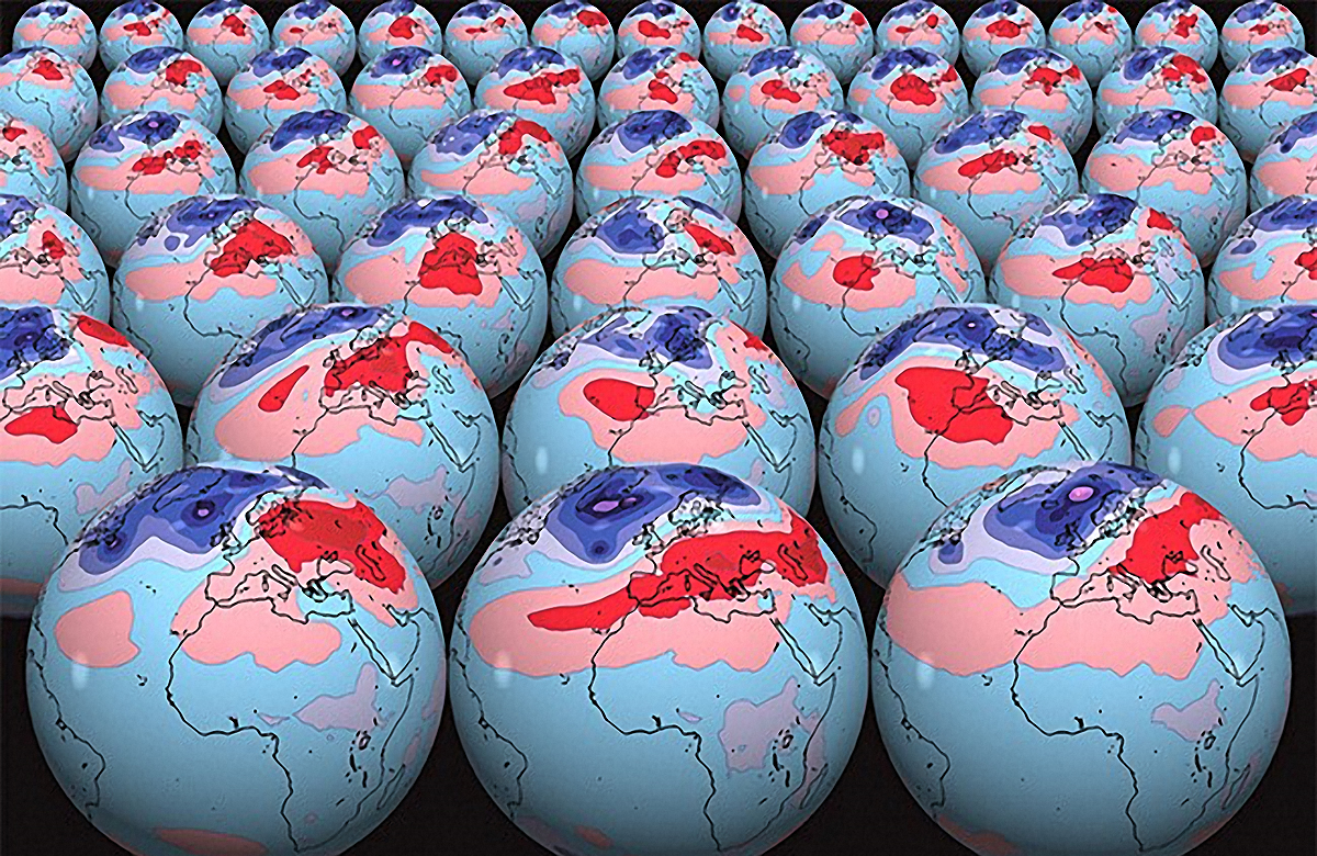
Take the weather, for instance. Small uncertainties in today’s weather—say, whether the temperature in Peoria at 2 pm was 78 degrees or 79 degrees—can become larger uncertainties tomorrow or a week from now. But computer weather models do a poor job of reproducing this effect. That’s because they use a legacy mathematical tool, called differential equations (in particular, the Navier-Stokes equations), that was designed to represent systems without including uncertainty.

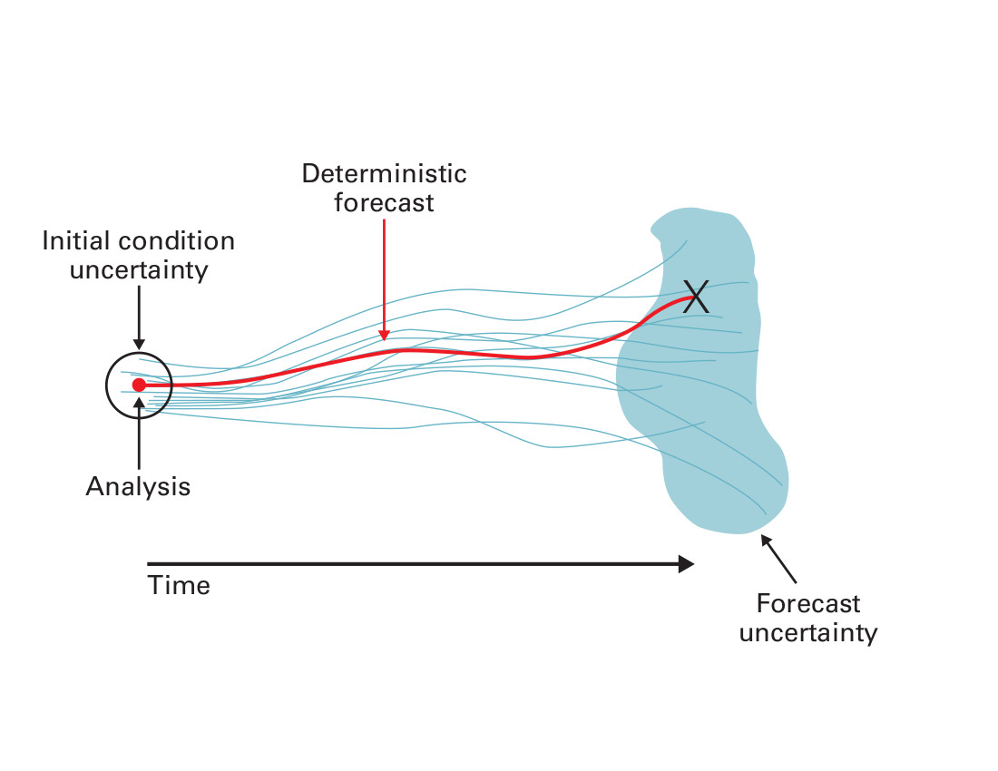
Weather forecasters know this, and they have a kludgy work-around. “They sample the weather in five or ten initial conditions and push each through the equations,” Venturi said. “Based on the outcome, they might say there is a 30 percent chance of rain. That just means that three simulations out of ten produced rain.”

We could call this approach “sample-then-propagate.” It’s a necessary kludge because differential equations can only transport points to points. If you give them the fog of a probability distribution as input, they don’t know what to do. Sample-then-propagate gives us pretty good weather forecasts. But it’s awkward and inefficient, and it does not deliver a representation with any guarantee of accuracy.

Ever since he was an undergraduate at the University of Bologna in Italy, Venturi has dreamed of building a tool that can actually solve the problem the right way: by transporting the fog of uncertainty from place to place or from time to time. He calls his method “functional differential equations” (FDE). But we can call it “propagate-then-sample.”

For math nerds, there is one difference between FDE and ordinary DE that is almost a showstopper. Ordinary DE involve finitely many variables, the dimensions of space and time that points move around in. But probability distributions live in an infinite-dimensional space because you can vary them in infinitely many different ways. “When I tell my colleagues I work on differential equations with infinitely many variables, they say, ‘Are you crazy?’” Venturi said. “That’s the biggest compliment I could get. It means it’s something interesting.”

Venturi traces the origins of FDE to Eberhard Hopf of Indiana University, who first used them in a theory of turbulence that dates from 1952. Russian mathematicians Andrei Monin and Akiva Yaglom revived them in 1971, calling Hopf’s equation “the most compact formulation of the general turbulence problem.” Functional differential equations were a perfect fit for studying turbulence because turbulent fluid flow cannot be predicted with certainty. Recently, though, FDEs are beginning to appear in disciplines not related to fluids.

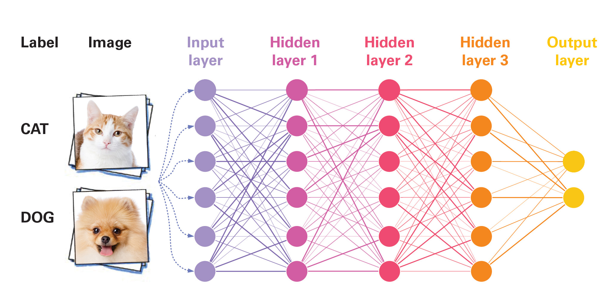
One surprising new example arises in machine learning. In recent years, deep neural networks—“deep” refers to a great number of layers—have had good success in realms like image recognition and computer chess and go. These networks loosely imitate the human brain, in which one layer of neurons might recognize individual pixels, while a deeper one pieces the pixels into curves, the next organizes them into trunk, limbs, and head, and the deepest layer finally recognizes the animal as a cat.

These complex constructs occupy the attention of mathematicians Weinan E and Jiequn Han at Princeton University, whose work explores the theoretical concept of a neural network with infinitely many layers. Such a network has to learn from essentially random input: a training set of images, some of which contain cats while others do not. It then needs to propagate uncertainty through all the layers of the network to obtain a classifier with (hopefully) the smallest amount of uncertainty possible. If this sounds to you like a problem made for FDE, you’ve passed the test.

That FDE is called a Hamilton-Jacobi-Bellman equation, and its solution is an operator that allows you to compute the weights—the strength of connections between layers—from any input. “It’s the core of how you train a neural network,” Venturi said.

Han said the advantage of “considering the problem in an infinite-dimensional space” is that it explains what neural networks are and why they work. They are discrete versions of a continuous, infinite-dimensional tool for propagating uncertainty. And, provided they are good approximations of such a hypothetical tool, they work well.

Venturi devotes a lot of effort to finding good discrete approximations to the solutions of FDE, in other words the second part of “propagate-then-sample.” In practice, this means solving some very high-dimensional (but not infinite) ordinary DE. It’s no longer “crazy,” but conventional, hard mathematics. “You need to know the state of the art really well to see if it is sufficient to achieve the goal you set at the beginning,” Venturi said. “The current state is insufficient. I don’t claim any victory, but what I do claim is a heroic attempt. The winner will be whoever is first able to compute the solutions well.”